Overview: in this blog post, we are going to be setting some of the theoretical foundations and intuition for the problems we think about. Over the coming week, we will release different blog posts focused on specific experiments and empirical questions. As such, this post aims to lay the groundwork for what's to come. We're excited to share the tip of the iceberg!

Language Models and Polysemanticity

The field of bottom-up mechanistic interpretability aims to elucidate the basic building blocks of machine cognition, which can be assembled hierarchically to build complex and emergent structures. In the early days of interpretability, researchers hypothesized that the fundamental unit of computation was the neuron and attempted to causally identify the role of individual neurons in early convolutional neural networks. These methods were met with limited success; researchers could occasionally cherry-pick one neuron or a set of neurons uniquely responsible for a task. However, the vast majority of the network did not appear to admit such a causal decomposition.

Roughly a year ago, Anthropic published Towards Monosemanticity, in which they explored the potential that the fundamental unit of computation in a neural network is a feature, which is a linear combination of neurons. Individual neurons, they argued, could play a role in representing multiple dissimilar features "in superposition," rendering them fundamentally uninterpretable.

Dictionary Learning & Sparsity

Dictionary learning provides a flexible, unsupervised method for learning large dictionaries of features (linear combinations of individual neurons). These dictionaries decompose the activations of a layer into a linear combination of features from the learned dictionary. The key insight is that by encouraging sparsity in this decomposition, we can obtain more interpretable and meaningful features.

Sparsity in this context means that only a small subset of the dictionary features are used to reconstruct any given activation. This approach has several advantages:

• Interpretable Features: Each feature (should) correspond to a specific, meaningful concept.
• Efficient Representation: Complex patterns can be represented using combinations of simpler elements.
• Denoising and Feature Extraction: By focusing on the most salient aspects of the data, representations have higher robustness.

The challenge lies in finding the right balance between sparsity and reconstruction accuracy. Too much sparsity can lead to the loss of important information, while too little may not provide the desired interpretability benefits and can lead to a high reconstruction error.

What Actually Makes Dictionary Learning Hard?

Navigating the sparsity-reconstruction Pareto frontier may seem like the primary concern with dictionary learning, but the real difficulty lies in the interpretability aspect. A good dictionary isn't necessarily interpretable, and vice versa.

The challenge of dictionary learning is further complicated by two key issues: the infinite width codebook problem and feature oversplitting.

An infinite-width codebook can trivially achieve optimal reconstruction with low sparsity by memorizing data examples. In this scenario, the dictionary becomes so large that it contains a unique feature for every possible input pattern. While this achieves perfect reconstruction and maintains sparsity (as each input is represented by a single feature), it fails to capture meaningful, generalizable patterns in the data. This approach defeats the true purpose of dictionary learning—to find a compact set of reusable features that can efficiently represent a wide range of inputs.

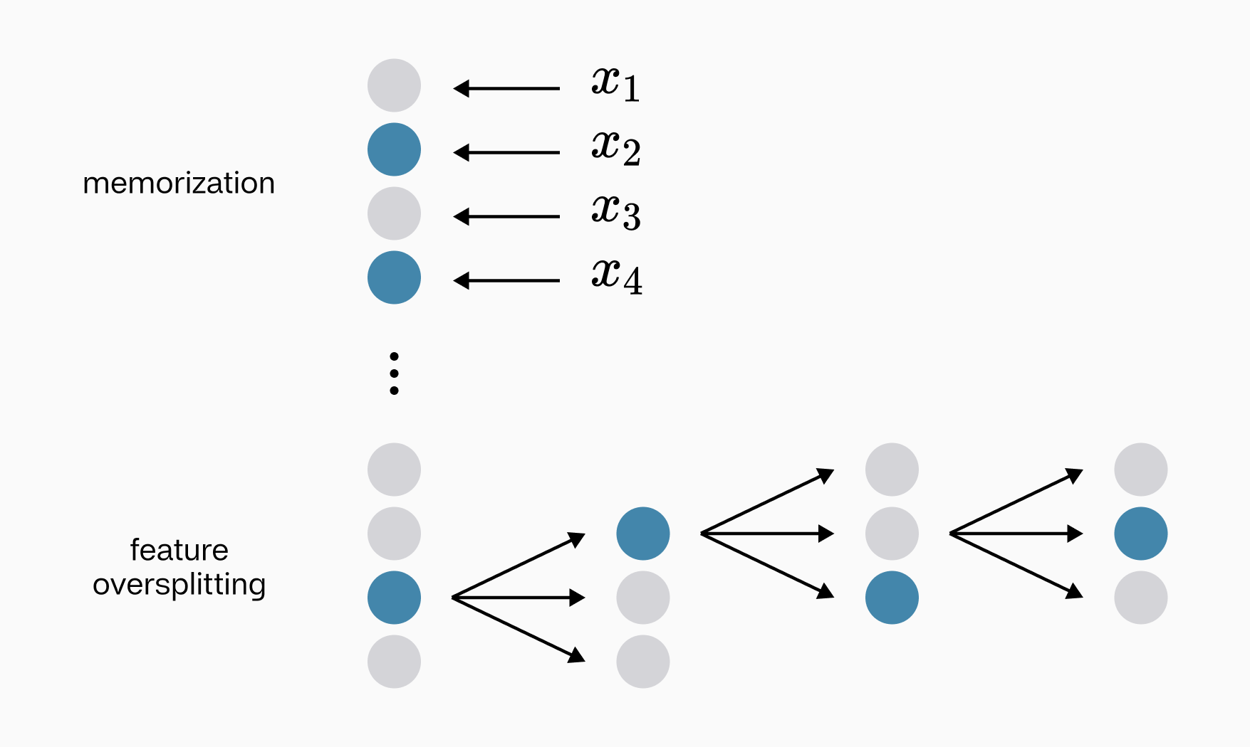Bigger dictionaries aren’t necessarily better - they fall victim to oversplitting and memorization. Making stronger dictionaries requires further insights.

On the other hand, feature oversplitting occurs when a network creates overly granular decision boundaries by splitting what should be cohesive features into multiple, highly specific ones. This problem arises because features are inherently amorphous and hierarchical concepts, while dictionaries are discrete and flat structures. For example, a feature representing "car" might be unnecessarily split into separate features for "red car," "blue car," and "green car." While this can lead to high reconstruction accuracy, it results in a less interpretable and generalizable dictionary.

These issues highlight the delicate balance required in dictionary learning. The goal is to find a set of features that are specific enough to accurately represent the data yet general enough to capture meaningful patterns and maintain interpretability. Achieving this balance often requires thoughtful regularization techniques and careful consideration of the dictionary size and learning algorithms employed.

A History of Sparsity

Sparsity is an easy concept to pin down intuitively but an elusive mathematical notion. When researchers discuss sparsity, they often implicitly impose the $\ell_0$ metric as the de facto measure. However, the history of sparse compression is deeply intertwined with our evolving understanding of data distributions and the priors we impose on them.

In the early days of signal processing, sparsity was often equated with having few non-zero elements. However, as our understanding deepened, researchers realized that sparsity is a more nuanced concept, heavily dependent on the assumptions we make about data.

Hurley and Rickard's 2009 paper, Comparing Measures of Sparsity, provides an excellent overview of how our understanding of sparsity has evolved. They discuss several different criteria for sparsity, including:

1. Robin Hood Index: This measure decreases sparsity by redistributing wealth (or signal energy) more evenly. It's based on the intuition that a sparse distribution has high inequality. 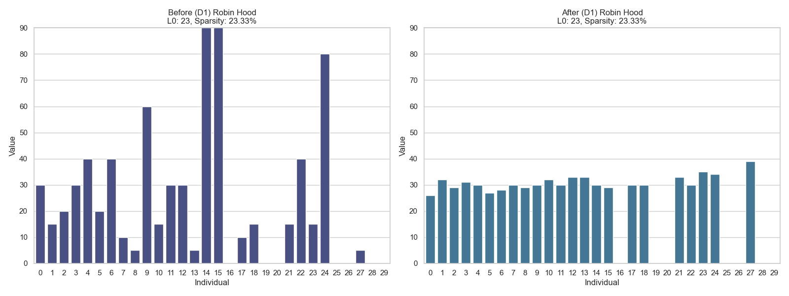❌ The $\ell_0$ norm remains unchanged when redistributing values since it only counts non-zero elements, not satisfying the Robin Hood Index criterion.

2. Scaling: Sparsity is considered scale-invariant. This reflects the prior that relative, not absolute, values determine sparsity. 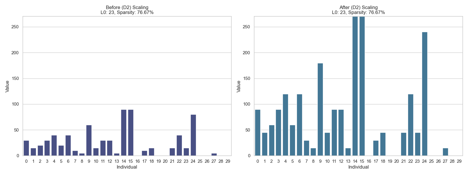✅ The $\ell_0$ norm is invariant to scaling since multiplying by a constant doesn't change which elements are non-zero, satisfying the Scaling criterion.

In general, they propose six measures, of which the $\ell_0$ norm only satisfies two!

Note: Due to space constraints, we won't delve into all six measures here, but interested readers are encouraged to consult Hurley and Rickard's paper for a comprehensive understanding.

The Encoder and The Decoder

Stepping back from the interpretability aspect, building an effective Sparse Autoencoder (SAE) involves addressing two fundamental problems: creating sparse codes that efficiently represent the data and accurately reconstructing the original data from these codes. The first job is tasked to the encoder matrix of the autoencoder, and the second to the decoder matrix. Fundamentally, these are problems in sparse coding theory and compressed sensing, respectively.

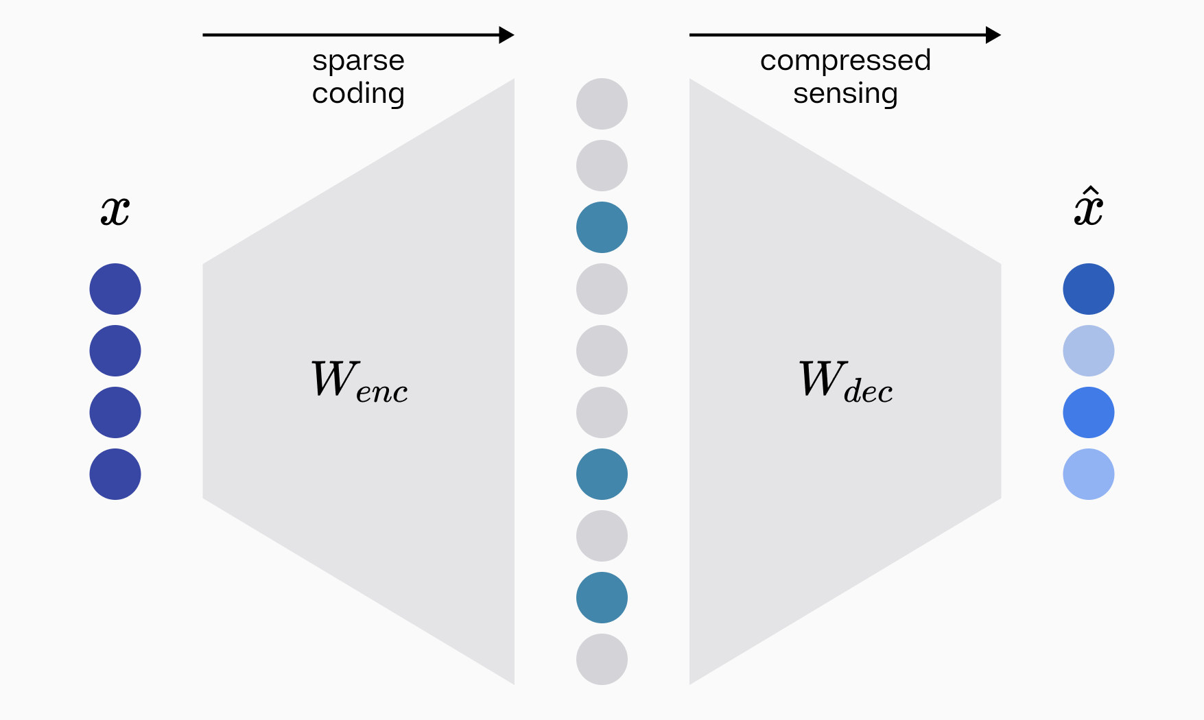The rate distortion dance of a sparse autoencoder can be broken down into two phases, sparse coding and compressed sensing, both of which have been studied classically for decades.

$W_{\text{enc}}$ and Sparse Coding Theory

The first component of the autoencoder is the encoder matrix—including the activation function—which falls directly within the field of sparse coding theory, originally introduced by Olshausen and Field (1996). The objective of sparse coding theory is to represent data as a sparse linear combination of basis elements. Formally, the mathematical goal of sparse coding is

where:

• $x \in \mathbb{R}^n$ is the input data vector,
• $D \in \mathbb{R}^{n \times k}$ is the dictionary matrix,
• $z \in \mathbb{R}^k$ is the sparse code,
• $\lambda$ is a regularization parameter balancing reconstruction fidelity and sparsity.

However, minimizing the $\ell_0$ norm is completely intractable due to its combinatorial nature, so the above equation is typically replaced with

which is easier to solve because the $\ell^1$ norm is convex.

This substitution raises the question: Is $\ell^1$ the best we can do? Are there other types of sparsity penalties that would yield better results? The answer is yes. For example, using a log-based sparsity penalty. In particular, it is well-known that $\ell^1$ is a generally poor approximation of $\ell_0$.

Another important discrepancy—which has also served as inspiration for newer SAE architectures—is the phenomenon of shrinkage. The $\ell^1$ sparsity penalty penalizes activation magnitudes uniformly, which pushes small values to zero but also has the unintended consequence of diminishing values that should be large. This is the primary complaint against the $\ell^1$ sparsity penalty and the motivation for other sparsity penalties.

Load Balancing

Furthermore, in sparse coding theory, as in a mixture of experts, we often consider the concept of load balancing. Load balancing refers to the even distribution of activations across different features or neurons in the sparse representation. In other words, having a code that fires evenly.

Prior work on SAEs, in particular top-k and JumpReLU architectures, has observed strong feature frequency misbalancing. Some features occur at disproportionately high frequency and are not interpretable, which is a failure of even feature allocation.

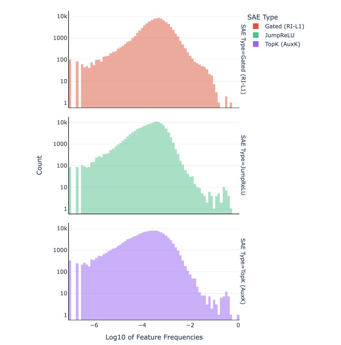Activation density histograms taken from Nanda et al (2024). High frequency features are on the right side.

Similar to sparsity, mechanisms of enforcing load balancing are fundamentally about stating and believing priors on how features should be behaving in the dataset (e.g. is it heavy-tailed?). However, if these high-frequency features are not a fundamental property of the model distribution (which certainly seems plausible), sparse coding-inspired load balancing regularization can help improve the interpretability of our dictionary.

Something we are really excited about, and are actively working on at Tilde, is alternative architectures informed by these types of ideas. Stay tuned for a more empirics-based blog post on this very soon :)

$W_{\text{dec}}$ and Compressed Sensing

Following the encoding process, the decoder matrix is tasked with reconstructing the original input $x$ from the sparse code $z$, a procedure within the realm of compressed sensing, which focuses on recovering high-dimensional signals from a small number of observations by exploiting sparsity.

Formally, in compressed sensing, one tries to solve

where:

• $y \in \mathbb{R}^m$ is the measurement vector,
• $A \in \mathbb{R}^{m \times n}$ is the measurement matrix,
• $x \in \mathbb{R}^n$ is the sparse signal to recover.

In our context, the decoder aims to reconstruct $x$ from $z$, analogous to recovering a signal from compressed measurements. The reconstruction can be thought of as:

To improve the decoder's performance, we can apply motivated ideas from compressed sensing. One such tactic is to impose an incoherence penalty on the columns of $W_{\text{dec}}$:

where:

• $\beta$ is a regularization parameter controlling the strength of the penalty,
• $W_{\text{dec}}^{(:,i)}$ denotes the $i$-th column of $W_{\text{dec}}$,
• $\langle \cdot , \cdot \rangle$ denotes the inner product.

The idea behind this penalty is to encourage the columns of $W_{\text{dec}}$ to be orthogonal or minimally correlated. This should enhance the decoder's ability to reconstruct the input effectively from sparse codes, as each column captures unique aspects of the data, and could improve the interpretability of the learned features.

Lastly, we'll examine Top-k through the lens of information bottleneck theory.

The Top-$k$ Activation Function in Sparse Autoencoders

When training a sparse autoencoder, the choice of activation function plays a crucial role in influencing the learning dynamics and sparsity of the dictionary.

Initially, one might consider activation functions like ReLU combined with $\ell^1$ regularization, treating dictionary learning as a multi-constraint problem where the network balances reconstruction error and sparsity penalties. In these architectures, sparsity is adaptive—some inputs may have more active latents if they are more complex to reconstruct, and vice versa.

However, Top-$k$ does away with this complexity! Instead of input-dependent sparsity, the sparsity of the latent vector is fixed for all inputs. Furthermore, instead of balancing a sparsity loss objective with reconstruction error, Top-$k$ sparse autoencoders only optimize for reconstruction error.

This raises an intriguing question: How can an approach that appears to reduce flexibility achieve strong performance gains over conventional methods? The answer lies in a concept central to sparse coding and compressed sensing—the Information Bottleneck (IB).

Squeezing Information Through the Information Bottleneck

The effectiveness of the Top-$k$ activation function in sparse autoencoders can be understood through the Information Bottleneck framework, which navigates a critical balance between information retention and compression. Formally, the IB principle seeks to encode a representation $Z$ of input $X$ that minimizes the mutual information $I(Z;X)$ while maximizing the relevance for reconstruction, $I(Z;Y)$:

where $\beta$ modulates the trade-off between compression and preservation of relevant information.

By fixing a constant number of active neurons across inputs, Top-$k$ directly enforces a ceiling on $I(Z;X)$, thus limiting the flow of information and naturally prioritizing the most informative features for reconstruction. Unlike traditional approaches that balance sparsity penalties and reconstruction, Top-$k$'s hard constraint simplifies this dynamic, optimizing exclusively for reconstruction accuracy within a set sparsity level.

The result is a built-in bottleneck effect: Top-$k$ reduces $I(Z;X)$ and potentially improves generalization by constraining information flow. This aligns with findings in generalization theory, which link model complexity to generalization error as:

where $n$ is the training sample size.

Essentially, Top-$k$ enforces a rate-distortion constraint, driving the network to prioritize stability and essential signal retention over noise. Indeed, in our experiments, Top-$k$ consistently produced smoother learning dynamics and greater robustness to noise compared to adaptive sparsity approaches.

Empirical studies in the IB framework show that neural networks often separate the training process into distinct phases, initially optimizing reconstruction and then enforcing sparsity. Our results echo this, finding that $\ell^1$ autoencoders first converge in reconstruction then undergo a long $\ell^1$ (and $\ell^0$) annealing phase with the reconstruction loss increasing. By contrast, Top-$k$'s stable sparsity constraint reduces sensitivity to early training noise, leading to more reliable convergence. While parameter tuning remains crucial, Top-$k$'s constrained information pathway allows for uniquely robust learning dynamics.

We trained top-k autoencoders on CIFAR10 for 50 epochs under different gaussian noising conditions. We hypothesized that the information bottleneck imposed by the architecture would improve robustness in high-noise settings.

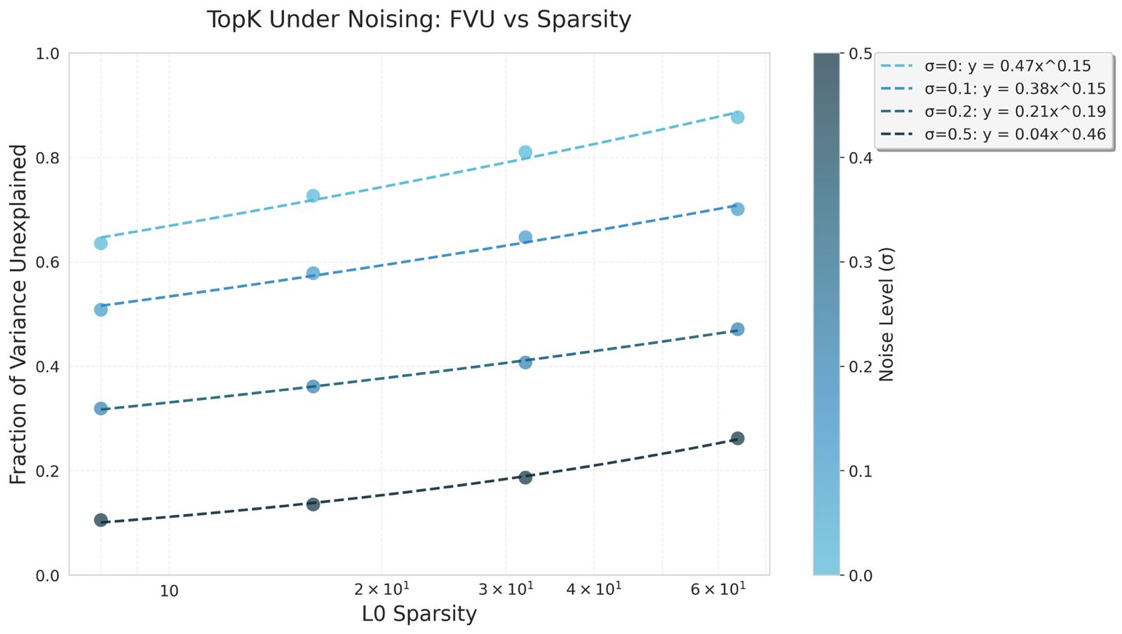Scaling laws of top-k under gaussian noise conditions. The information bottleneck improves the robustness of top-k.

The coefficient of the power law fit for top-k increased in higher noise regimes, implying larger k values may better recover signal from the noise. Furthermore, training dynamics were highly stable and had almost monotonic convergence in loss. Our implementations of ReLU baselines tested on high noise settings collapsed/diverged and as such we excluded them from the graph.

Conclusion

At Tilde, we're excited about these ideas and are actively incorporating them into the interpreter models that we train. There are decades of mathematical insights in compressed sensing and sparse coding that we're just beginning to scratch the surface of, and we're looking forward to exploring them further.

Stay tuned for more empirically focused updates in our upcoming blog posts!

References:

• Olshausen, B. A., & Field, D. J. (1996). Emergence of simple-cell receptive field properties by learning a sparse code for natural images
• Hurley, N., & Rickard, S. (2009). Comparing measures of sparsity
• Bricken et. al. (2024). Towards Monosemanticity: Decomposing Language Models With Dictionary Learning
• Gao et. al. (2024). Scaling and Evaluating Sparse Autoencoders
• Rajamanoharan et. al. (2024). Jumping Ahead: Improving Reconstruction Fidelity with JumpReLU Sparse Autoencoders
• Kawaguchi et. al (2023) How Does Information Bottleneck Help Deep Learning?

References

- Olshausen, Bruno, and Field, David (1996).
- Hurley, Niall and Rickard, Scott (2009).
- Bricken, Trenton and Templeton, Adly and Batson, Joshua and Chen, Brian and Jermyn, Adam and Conerly, Tom and Turner, Nick and Anil, Cem and Denison, Carson and Askell, Amanda and Lasenby, Robert and Wu, Yifan and Kravec, Shauna and Schiefer, Nicholas and Maxwell, Tim and Joseph, Nicholas and Hatfield-Dodds, Zac and Tamkin, Alex and Nguyen, Karina and McLean, Brayden and Burke, Josiah E and Hume, Tristan and Carter, Shan and Henighan, Tom and Olah, Christopher (2023).
- Gao, Leo and Dupré la Tour, Tom and Tillman, Henk and Goh, Gabriel and Troll, Rajan and Radford, Alec and Sutskever, Ilya and Leike, Jan and Wu, Jeffrey (2024).
- Senthooran Rajamanoharan, Tom Lieberum, Nicolas Sonnerat, Arthur Conmy, Vikrant Varma, János Kramár, Neel Nanda (2024).
- Kenji Kawaguchi, Zhun Deng, Xu Ji, Jiaoyang Huang (2023).